Chapter 1 Introduction to R
1.1 Getting Started
R is both a programming language and software environment for statistical computing, which is free and open-source. To get started, you will need to install two pieces of software:
R, the actual programming language.- Chose your operating system, and select the most recent version.
- RStudio, an excellent IDE for working with
R.- Note, you must have
Rinstalled to use RStudio. RStudio is simply an interface used to interact withR.
- Note, you must have
The popularity of R is on the rise, and everyday it becomes a better tool for statistical analysis. It even generated this book!
The following few chapters will serve as a whirlwind introduction to R. They are by no means meant to be a complete reference for the R language, but simply an introduction to the basics that we will need along the way. Several of the more important topics will be re-stressed as they are actually needed for analyses.
This introductory R chapter may feel like an overwhelming amount of information. You are not expected to pick up everything the first time through. You should try all of the code from this chapter, then return to it a number of times as you return to the concepts when performing analyses. We only present the most basic aspects of R. If you want to know more, there are countless online tutorials, and you could start with the official CRAN sample session or have a look at the resources at Rstudio or on this github repo.
1.2 Starting R and RStudio
A key difference for you to understand is the one between R, the actual programming language, and RStudio, a popular interface to R which allows you to work efficiently and with greater ease with R.
The best way to appreciate the value of RStudio is to start using R without RStudio. To do this, double-click on the R GUI that you should have downloaded on your computer following the steps above (on windows or Mac), or start R in your terminal (on Linux or Mac) by just typing R in a terminal, see figure ??. You’ve just opened the R console which allows you to start typing code right after the > sign, called prompt. Try typing 2 + 2 or print("Your Name") and hit the return key. And voilà, your first R commands!

Figure 1.1: R GUI symbol and R in a MacOS Terminal
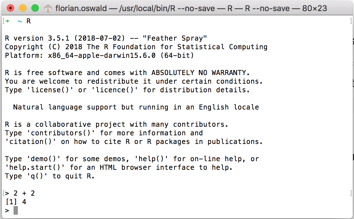
Figure 1.2: R GUI symbol and R in a MacOS Terminal
Typing one command after the other into the console is not very convenient as our analysis becomes more involved. Ideally, we would like to collect all command statements in a file and run them one after the other, automatically. We can do this by writing so-called script files or just scripts, i.e. simple text files with extension .R or .r which can be inserted (or sourced) into an R session. RStudio makes this process very easy.
Open RStudio by clicking on the RStudio application on your computer, and notice how different the whole environment is from the basic R console – in fact, that very same R console is running in your bottom left panel. The upper-left panel is a space for you to write scripts – that is to say many lines of codes which you can run when you choose to. To run a single line of code, simply highlight it and hit Command + Return.
We highly recommend that you use RStudio for everything related to this course (in particular, to launch our apps and tutorials).
RStudio has a large number of useful keyboard shortcuts. A list of these can be found using a keyboard shortcut – the keyboard shortcut to rule them all:
- On Windows:
Alt+Shift+K - On Mac:
Option+Shift+K
The RStudio team has developed a number of “cheatsheets” for working with both R and RStudio. This particular cheatseet for Base R will summarize many of the concepts in this document.1
1.2.1 First Glossary
R: a statistical programming languageRStudio: an integrated development environment (IDE) to work withR- command: user input (text or numbers) that
Runderstands. - script: a list of commands collected in a text file, each separated by a new line, to be run one after the other.
1.3 Basic Calculations
To get started, we’ll use R like a simple calculator. Run the following code either directly from your RStudio console, or in RStudio by writting them in a script and running them using Command + Return.
Addition, Subtraction, Multiplication and Division
| Math | R code |
Result |
|---|---|---|
| \(3 + 2\) | 3 + 2 |
5 |
| \(3 - 2\) | 3 - 2 |
1 |
| \(3 \cdot2\) | 3 * 2 |
6 |
| \(3 / 2\) | 3 / 2 |
1.5 |
Exponents
| Math | R code |
Result |
|---|---|---|
| \(3^2\) | 3 ^ 2 |
9 |
| \(2^{(-3)}\) | 2 ^ (-3) |
0.125 |
| \(100^{1/2}\) | 100 ^ (1 / 2) |
10 |
| \(\sqrt{100}\) | sqrt(100) |
10 |
Mathematical Constants
| Math | R code |
Result |
|---|---|---|
| \(\pi\) | pi |
3.1415927 |
| \(e\) | exp(1) |
2.7182818 |
Logarithms
Note that we will use \(\ln\) and \(\log\) interchangeably to mean the natural logarithm. There is no ln() in R, instead it uses log() to mean the natural logarithm.
| Math | R code |
Result |
|---|---|---|
| \(\log(e)\) | log(exp(1)) |
1 |
| \(\log_{10}(1000)\) | log10(1000) |
3 |
| \(\log_{2}(8)\) | log2(8) |
3 |
| \(\log_{4}(16)\) | log(16, base = 4) |
2 |
Trigonometry
| Math | R code |
Result |
|---|---|---|
| \(\sin(\pi / 2)\) | sin(pi / 2) |
1 |
| \(\cos(0)\) | cos(0) |
1 |
1.4 Getting Help
In using R as a calculator, we have seen a number of functions: sqrt(), exp(), log() and sin(). To get documentation about a function in R, simply put a question mark in front of the function name, or call the function help(function) and RStudio will display the documentation, for example:
?log
?sin
?paste
?lm
help(lm)   # help() is equivalent
help(ggplot,package="ggplot2")  # show help from a certain package
Frequently one of the most difficult things to do when learning R is asking for help. First, you need to decide to ask for help, then you need to know how to ask for help. Your very first line of defense should be to Google your error message or a short description of your issue. (The ability to solve problems using this method is quickly becoming an extremely valuable skill.) If that fails, and it eventually will, you should ask for help. There are a number of things you should include when contacting an instructor, or posting to a help website such as Stack Overflow.
- Describe what you expect the code to do.
- State the end goal you are trying to achieve. (Sometimes what you expect the code to do, is not what you want to actually do.)
- Provide the full text of any errors you have received.
- Provide enough code to recreate the error. Often for the purpose of this course, you could simply post your entire
.Rscript or.Rmdtoslack. - Sometimes it is also helpful to include a screenshot of your entire RStudio window when the error occurs.
If you follow these steps, you will get your issue resolved much quicker, and possibly learn more in the process. Do not be discouraged by running into errors and difficulties when learning R. (Or any other technical skill.) It is simply part of the learning process.
1.5 Installing Packages
R comes with a number of built-in functions and datasets, but one of the main strengths of R as an open-source project is its package system. Packages add additional functions and data. Frequently if you want to do something in R, and it is not available by default, there is a good chance that there is a package that will fulfill your needs.
To install a package, use the install.packages() function. Think of this as buying a recipe book from the store, bringing it home, and putting it on your shelf (i.e. into your library):
Once a package is installed, it must be loaded into your current R session before being used. Think of this as taking the book off of the shelf and opening it up to read.
Once you close R, all the packages are closed and put back on the imaginary shelf. The next time you open R, you do not have to install the package again, but you do have to load any packages you intend to use by invoking library().
1.6 Code vs Output in this Book
A quick note on styling choices in this book. We had to make a decision how to visually separate R code and resulting output in this book. All output lines are prefixed with ## to make the distinction. A typical code snippet with output is thus going to look like this:
## [1] 4where you see on the first line the R code, and on the second line the output. As mentioned, that line starts with ## to say this is an output, followed by [1] (indicating this is a vector of length one - more on this below!), followed by the actual result - 1 + 3 = 4!
Notice that you can simply copy and paste all the code you see into your R console. In fact, you are strongly encouraged to actually do this and try out all the code you see in this book.
Finally, please note that this way of showing output is fully our choice in this textbook, and that you should expect other output formats elsewhere. For example, in my RStudio console, the above code and output looks like this:
1.7 ScPoApps Package
To fully take advantage of our course, please install the associated R package directly from its online code repository. You can do this by copy and pasting the following three lines into your R console:
if (!require("devtools")) install.packages("devtools")
devtools::install_github(repo = "ScPoEcon/ScPoApps")
In order to check whether everything works fine, you could load the library, and check it’s current version:
1.8 Data Types
R has a number of basic data types. While R is not a strongly typed language (i.e. you can be agnostic about types most of the times), it is useful to know what data types are available to you:
- Numeric
- Also known as Double. The default type when dealing with numbers.
- Examples:
1,1.0,42.5
- Integer
- Examples:
1L,2L,42L
- Examples:
- Complex
- Example:
4 + 2i
- Example:
- Logical
- Two possible values:
TRUEandFALSE - You can also use
TandF, but this is not recommended. NAis also considered logical.
- Two possible values:
- Character
- Examples:
"a","Statistics","1 plus 2."
- Examples:
- Categorical or
factor- A mixture of integer and character. A
factorvariable assigns a label to a numeric value. - For example
factor(x=c(0,1),labels=c("male","female"))assigns the string male to the numeric values0, and the string female to the value1.
- A mixture of integer and character. A
1.9 Data Structures
R also has a number of basic data structures. A data structure is either homogeneous (all elements are of the same data type) or heterogeneous (elements can be of more than one data type).
| Dimension | Homogeneous | Heterogeneous |
|---|---|---|
| 1 | Vector | List |
| 2 | Matrix | Data Frame |
| 3+ | Array | nested Lists |
1.9.1 Vectors
Many operations in R make heavy use of vectors. A vector is a container for objects of identical type (see 1.8 above). Vectors in R are indexed starting at 1. That is what the [1] in the output is indicating, that the first element of the row being displayed is the first element of the vector. Larger vectors will start additional rows with something like [7] where 7 is the index of the first element of that row.
Possibly the most common way to create a vector in R is using the c() function, which is short for “combine”. As the name suggests, it combines a list of elements separated by commas. (Are you busy typing all of those examples into your R console? :-) )
## [1] 1 3 5 7 8 9Here R simply outputs this vector. If we would like to store this vector in a variable we can do so with the assignment operator =. In this case the variable x now holds the vector we just created, and we can access the vector by typing x.
## [1] 1 3 5 7 8 9As an aside, there is a long history of the assignment operator in R, partially due to the keys available on the keyboards of the creators of the S language. (Which preceded R.) For simplicity we will use =, but know that often you will see <- as the assignment operator.
Because vectors must contain elements that are all the same type, R will automatically coerce (i.e. convert) to a single type when attempting to create a vector that combines multiple types.
## [1] "42" "Statistics" "TRUE"## [1] 42 1Frequently you may wish to create a vector based on a sequence of numbers. The quickest and easiest way to do this is with the : operator, which creates a sequence of integers between two specified integers.
##   [1]   1   2   3   4   5   6   7   8   9  10  11  12  13  14  15  16  17  18
##  [19]  19  20  21  22  23  24  25  26  27  28  29  30  31  32  33  34  35  36
##  [37]  37  38  39  40  41  42  43  44  45  46  47  48  49  50  51  52  53  54
##  [55]  55  56  57  58  59  60  61  62  63  64  65  66  67  68  69  70  71  72
##  [73]  73  74  75  76  77  78  79  80  81  82  83  84  85  86  87  88  89  90
##  [91]  91  92  93  94  95  96  97  98  99 100
Here we see R labeling the rows after the first since this is a large vector. Also, we see that by putting parentheses around the assignment, R both stores the vector in a variable called y and automatically outputs y to the console.
Note that scalars do not exists in R. They are simply vectors of length 1.
## [1] 2If we want to create a sequence that isn’t limited to integers and increasing by 1 at a time, we can use the seq() function.
##  [1] 1.5 1.6 1.7 1.8 1.9 2.0 2.1 2.2 2.3 2.4 2.5 2.6 2.7 2.8 2.9 3.0 3.1 3.2 3.3
## [20] 3.4 3.5 3.6 3.7 3.8 3.9 4.0 4.1 4.2
We will discuss functions in detail later, but note here that the input labels from, to, and by are optional.
##  [1] 1.5 1.6 1.7 1.8 1.9 2.0 2.1 2.2 2.3 2.4 2.5 2.6 2.7 2.8 2.9 3.0 3.1 3.2 3.3
## [20] 3.4 3.5 3.6 3.7 3.8 3.9 4.0 4.1 4.2
Another common operation to create a vector is rep(), which can repeat a single value a number of times.
## [1] "A" "A" "A" "A" "A" "A" "A" "A" "A" "A"The rep() function can be used to repeat a vector some number of times.
## [1] 1 3 5 7 8 9 1 3 5 7 8 9 1 3 5 7 8 9We have now seen four different ways to create vectors:
c():seq()rep()
So far we have mostly used them in isolation, but they are often used together.
##  [1]  1  3  5  7  8  9  1  3  5  7  9  1  3  5  7  9  1  3  5  7  9  1  2  3 42
## [26]  2  3  4
The length of a vector can be obtained with the length() function.
## [1] 6## [1] 100Let’s try this out! Your turn:
1.9.1.1 Task 1
- Create a vector of five ones, i.e.
[1,1,1,1,1] - Notice that the colon operator
a:bis just short for construct a sequence fromatob. Create a vector the counts down from 10 to 0, i.e. it looks like[10,9,8,7,6,5,4,3,2,1,0]! - the
repfunction takes additional argumentstimes(as above), andeach, which tells you how often each element should be repeated (as opposed to the entire input vector). Userepto create a vector that looks like this:[1 1 1 2 2 2 3 3 3 1 1 1 2 2 2 3 3 3]
1.9.1.2 Subsetting
To subset a vector, i.e. to choose only some elements of it, we use square brackets, []. Here we see that x[1] returns the first element, and x[3] returns the third element:
## [1] 1 3 5 7 8 9## [1] 1## [1] 5We can also exclude certain indexes, in this case the second element.
## [1] 1 5 7 8 9Lastly we see that we can subset based on a vector of indices.
## [1] 1 3 5## [1] 1 5 7All of the above are subsetting a vector using a vector of indexes. (Remember a single number is still a vector.) We could instead use a vector of logical values.
## [1] TRUE TRUE FALSE TRUE TRUE FALSE## [1] 1 3 7 8R is able to perform many operations on vectors and scalars alike:
## [1] 2 3 4 5 6 7 8 9 10 11## [1] 2 4 6 8 10 12 14 16 18 20## [1] 2 4 8 16 32 64 128 256 512 1024## [1] 1.000000 1.414214 1.732051 2.000000 2.236068 2.449490 2.645751 2.828427
## [9] 3.000000 3.162278## [1] 0.0000000 0.6931472 1.0986123 1.3862944 1.6094379 1.7917595 1.9459101
## [8] 2.0794415 2.1972246 2.3025851## [1] 3 6 9 12 15 18 21 24 27 30We see that when a function like log() is called on a vector x, a vector is returned which has applied the function to each element of the vector x.
1.9.2 Logical Operators
| Operator | Summary | Example | Result |
|---|---|---|---|
x < y |
x less than y |
3 < 42 |
TRUE |
x > y |
x greater than y |
3 > 42 |
FALSE |
x <= y |
x less than or equal to y |
3 <= 42 |
TRUE |
x >= y |
x greater than or equal to y |
3 >= 42 |
FALSE |
x == y |
xequal to y |
3 == 42 |
FALSE |
x != y |
x not equal to y |
3 != 42 |
TRUE |
!x |
not x |
!(3 > 42) |
TRUE |
x | y |
x or y |
(3 > 42) | TRUE |
TRUE |
x & y |
x and y |
(3 < 4) & ( 42 > 13) |
TRUE |
In R, logical operators also work on vectors:
## [1] FALSE FALSE TRUE TRUE TRUE TRUE## [1] TRUE FALSE FALSE FALSE FALSE FALSE## [1] FALSE TRUE FALSE FALSE FALSE FALSE## [1] TRUE FALSE TRUE TRUE TRUE TRUE## [1] FALSE FALSE FALSE FALSE FALSE FALSE## [1] TRUE TRUE TRUE TRUE TRUE TRUEThis is quite useful for subsetting.
## [1] 5 7 8 9## [1] 1 5 7 8 9## [1] 4## [1] 0 0 1 1 1 1Here we saw that using the sum() function on a vector of logical TRUE and FALSE values that is the result of x > 3 results in a numeric result: you just counted for how many elements of x, the condition > 3 is TRUE. During the call to sum(), R is first automatically coercing the logical to numeric where TRUE is 1 and FALSE is 0. This coercion from logical to numeric happens for most mathematical operations.
## [1] 3 4 5 6## [1] 5 7 8 9## [1] 9## [1] 6## [1] 61.9.2.1 Task 2
- Create a vector filled with 10 numbers drawn from the uniform distribution (hint: use function
runif) and store them inx. - Using logical subsetting as above, get all the elements of
xwhich are larger than 0.5, and store them iny. - using the function
which, store the indices of all the elements ofxwhich are larger than 0.5 iniy. - Check that
yandx[iy]are identical.
1.9.3 Matrices
R can also be used for matrix calculations. Matrices have rows and columns containing a single data type. In a matrix, the order of rows and columns is important. (This is not true of data frames, which we will see later.)
Matrices can be created using the matrix function.
## [1] 1 2 3 4 5 6 7 8 9## [,1] [,2] [,3]
## [1,] 1 4 7
## [2,] 2 5 8
## [3,] 3 6 9Notice here that R is case sensitive (x vs X).
By default the matrix function fills your data into the matrix column by column. But we can also tell R to fill rows instead:
## [,1] [,2] [,3]
## [1,] 1 2 3
## [2,] 4 5 6
## [3,] 7 8 9We can also create a matrix of a specified dimension where every element is the same, in this case 0.
## [,1] [,2] [,3] [,4]
## [1,] 0 0 0 0
## [2,] 0 0 0 0Like vectors, matrices can be subsetted using square brackets, []. However, since matrices are two-dimensional, we need to specify both a row and a column when subsetting.
##      [,1] [,2] [,3]
## [1,]    1    4    7
## [2,]    2    5    8
## [3,] 3 6 9## [1] 4Here we accessed the element in the first row and the second column. We could also subset an entire row or column.
## [1] 1 4 7## [1] 4 5 6We can also use vectors to subset more than one row or column at a time. Here we subset to the first and third column of the second row:
## [1] 2 8Matrices can also be created by combining vectors as columns, using cbind, or combining vectors as rows, using rbind.
## [1] 9 8 7 6 5 4 3 2 1## [1] 1 1 1 1 1 1 1 1 1## [,1] [,2] [,3] [,4] [,5] [,6] [,7] [,8] [,9]
## x 1 2 3 4 5 6 7 8 9
## 9 8 7 6 5 4 3 2 1
## 1 1 1 1 1 1 1 1 1## col_1 col_2 col_3
## [1,] 1 9 1
## [2,] 2 8 1
## [3,] 3 7 1
## [4,] 4 6 1
## [5,] 5 5 1
## [6,] 6 4 1
## [7,] 7 3 1
## [8,] 8 2 1
## [9,] 9 1 1When using rbind and cbind you can specify “argument” names that will be used as column names.
R can then be used to perform matrix calculations.
##      [,1] [,2] [,3]
## [1,]    1    4    7
## [2,]    2    5    8
## [3,] 3 6 9## [,1] [,2] [,3]
## [1,] 9 6 3
## [2,] 8 5 2
## [3,] 7 4 1## [,1] [,2] [,3]
## [1,] 10 10 10
## [2,] 10 10 10
## [3,] 10 10 10## [,1] [,2] [,3]
## [1,] -8 -2 4
## [2,] -6 0 6
## [3,] -4 2 8## [,1] [,2] [,3]
## [1,] 9 24 21
## [2,] 16 25 16
## [3,] 21 24 9## [,1] [,2] [,3]
## [1,] 0.1111111 0.6666667 2.333333
## [2,] 0.2500000 1.0000000 4.000000
## [3,] 0.4285714 1.5000000 9.000000Note that X * Y is not matrix multiplication. It is element by element multiplication. (Same for X / Y).
Matrix multiplication uses %*%. Other matrix functions include t() which gives the transpose of a matrix and solve() which returns the inverse of a square matrix if it is invertible.
##      [,1] [,2] [,3]
## [1,]   90   54   18
## [2,]  114   69   24
## [3,] 138 84 30## [,1] [,2] [,3]
## [1,] 1 2 3
## [2,] 4 5 6
## [3,] 7 8 91.9.4 Arrays
A vector is a one-dimensional array. A matrix is a two-dimensional array. In R you can create arrays of arbitrary dimensionality N. Here is how:
d = 1:16
d3 = array(data = d,dim = c(4,2,2))
d4 = array(data = d,dim = c(4,2,2,3))  # will recycle 1:16
d3
## , , 1
##
## [,1] [,2]
## [1,] 1 5
## [2,] 2 6
## [3,] 3 7
## [4,] 4 8
##
## , , 2
##
## [,1] [,2]
## [1,] 9 13
## [2,] 10 14
## [3,] 11 15
## [4,] 12 16You can see that d3 are simply two (4,2) matrices laid on top of each other, as if there were two pages. Similary, d4 would have two pages, and another 3 registers in a fourth dimension. And so on.
You can subset an array like you would a vector or a matrix, taking care to index each dimension:
## [1] 1 2 3 4## , , 1
##
## [,1] [,2]
## [1,] 2 6
## [2,] 3 7
##
## , , 2
##
## [,1] [,2]
## [1,] 10 14
## [2,] 11 15## [1] 6 141.9.4.1 Task 3
- Create a vector containing
1,2,3,4,5called v. - Create a (2,5) matrix
mcontaining the data1,2,3,4,5,6,7,8,9,10. The first row should be1,2,3,4,5. - Perform matrix multiplication of
mwithv. Use the command%*%. What dimension does the output have? - Why does
v %*% mnot work?
1.9.5 Lists
A list is a one-dimensional heterogeneous data structure. So it is indexed like a vector with a single integer value (or with a name), but each element can contain an element of any type. Lists are similar to a python or julia Dict object. Many R structures and outputs are lists themselves. Lists are extremely useful and versatile objects, so make sure you understand their useage:
## [[1]]
## [1] 42
##
## [[2]]
## [1] "Hello"
##
## [[3]]
## [1] TRUE
# creation with fieldnames
ex_list = list(
a = c(1, 2, 3, 4),
b = TRUE,
c = "Hello!",
d = function(arg = 42) {print("Hello World!")},
e = diag(5)
)Lists can be subset using two syntaxes, the $ operator, and square brackets []. The $ operator returns a named element of a list. The [] syntax returns a list, while the [[]] returns an element of a list.
ex_list[1]returns a list contain the first element.ex_list[[1]]returns the first element of the list, in this case, a vector.
##      [,1] [,2] [,3] [,4] [,5]
## [1,]    1    0    0    0    0
## [2,]    0    1    0    0    0
## [3,]    0    0    1    0    0
## [4,]    0    0    0    1    0
## [5,] 0 0 0 0 1## $a
## [1] 1 2 3 4
##
## $b
## [1] TRUE## $a
## [1] 1 2 3 4## [1] 1 2 3 4## $e
## [,1] [,2] [,3] [,4] [,5]
## [1,] 1 0 0 0 0
## [2,] 0 1 0 0 0
## [3,] 0 0 1 0 0
## [4,] 0 0 0 1 0
## [5,] 0 0 0 0 1
##
## $a
## [1] 1 2 3 4## $e
##      [,1] [,2] [,3] [,4] [,5]
## [1,]    1    0    0    0    0
## [2,]    0    1    0    0    0
## [3,]    0    0    1    0    0
## [4,]    0    0    0    1    0
## [5,] 0 0 0 0 1## [,1] [,2] [,3] [,4] [,5]
## [1,] 1 0 0 0 0
## [2,] 0 1 0 0 0
## [3,] 0 0 1 0 0
## [4,] 0 0 0 1 0
## [5,] 0 0 0 0 1## function(arg = 42) {print("Hello World!")}## [1] "Hello World!"1.9.5.1 Task 4
- Copy and paste the above code for
ex_listinto your R session. Remember thatlistcan hold any kind ofRobject. Like…another list! So, create a new listnew_listthat has two fields: a first field called “this” with string content"is awesome", and a second field called “ex_list” that containsex_list. - Accessing members is like in a plain list, just with several layers now. Get the element
cfromex_listinnew_list! - Compose a new string out of the first element in
new_list, the element under labelthis. Use the functionpasteto printR is awesometo your screen.
1.10 Data Frames
We have previously seen vectors and matrices for storing data as we introduced R. We will now introduce a data frame which will be the most common way that we store and interact with data in this course. A data.frame is similar to a python pandas.dataframe or a julia DataFrame. (But the R version was the first! :-) )
example_data = data.frame(x = c(1, 3, 5, 7, 9, 1, 3, 5, 7, 9),
                          y = c(rep("Hello", 9), "Goodbye"),
                          z = rep(c(TRUE, FALSE), 5))
Unlike a matrix, which can be thought of as a vector rearranged into rows and columns, a data frame is not required to have the same data type for each element. A data frame is a list of vectors, and each vector has a name. So, each vector must contain the same data type, but the different vectors can store different data types. Note, however, that all vectors must have the same length (differently from a list)!
A data.frame is similar to a typical Spreadsheet. There are rows, and there are columns. A row is typically thought of as an observation, and each column is a certain variable, characteristic or feature of that observation.
Let’s look at the data frame we just created above:
##    x       y     z
## 1  1   Hello  TRUE
## 2  3   Hello FALSE
## 3  5   Hello  TRUE
## 4  7   Hello FALSE
## 5  9   Hello  TRUE
## 6  1   Hello FALSE
## 7  3   Hello  TRUE
## 8  5   Hello FALSE
## 9  7   Hello  TRUE
## 10 9 Goodbye FALSE
Unlike a list, which has more flexibility, the elements of a data frame must all be vectors. Again, we access any given column with the $ operator:
## [1] 1 3 5 7 9 1 3 5 7 9## [1] TRUE## 'data.frame': 10 obs. of 3 variables:
## $ x: num 1 3 5 7 9 1 3 5 7 9
## $ y: chr "Hello" "Hello" "Hello" "Hello" ...
## $ z: logi TRUE FALSE TRUE FALSE TRUE FALSE ...## [1] 10## [1] 3## [1] 10 3## [1] "x" "y" "z"1.10.1 Working with data.frames
The data.frame() function above is one way to create a data frame. We can also import data from various file types in into R, as well as use data stored in packages.
To read this data back into R, we will use the built-in function read.csv:
path = system.file(package="ScPoEconometrics","datasets","example-data.csv")
example_data_from_disk = read.csv(path)
This particular line of code assumes that you installed the associated R package to this book, hence you have this dataset stored on your computer at system.file(package = "ScPoEconometrics","datasets","example-data.csv").
##    x       y     z
## 1  1   Hello  TRUE
## 2  3   Hello FALSE
## 3  5   Hello  TRUE
## 4  7   Hello FALSE
## 5  9   Hello  TRUE
## 6  1   Hello FALSE
## 7  3   Hello  TRUE
## 8  5   Hello FALSE
## 9  7   Hello  TRUE
## 10 9 Goodbye FALSE
When using data, there are three things we would generally like to do:
- Look at the raw data.
- Understand the data. (Where did it come from? What are the variables? Etc.)
- Visualize the data.
To look at data in a data.frame, we have two useful commands: head() and str().
##                      mpg cyl  disp  hp drat    wt  qsec vs am gear carb
## Mazda RX4           21.0   6 160.0 110 3.90 2.620 16.46  0  1    4    4
## Mazda RX4 Wag       21.0   6 160.0 110 3.90 2.875 17.02  0  1    4    4
## Datsun 710          22.8   4 108.0  93 3.85 2.320 18.61  1  1    4    1
## Hornet 4 Drive      21.4   6 258.0 110 3.08 3.215 19.44  1  0    3    1
## Hornet Sportabout   18.7   8 360.0 175 3.15 3.440 17.02  0  0    3    2
## Valiant             18.1   6 225.0 105 2.76 3.460 20.22  1  0    3    1
## Duster 360          14.3   8 360.0 245 3.21 3.570 15.84  0  0    3    4
## Merc 240D           24.4   4 146.7  62 3.69 3.190 20.00  1  0    4    2
## Merc 230            22.8   4 140.8  95 3.92 3.150 22.90  1  0    4    2
## Merc 280            19.2   6 167.6 123 3.92 3.440 18.30  1  0    4    4
## Merc 280C           17.8   6 167.6 123 3.92 3.440 18.90  1  0    4    4
## Merc 450SE          16.4   8 275.8 180 3.07 4.070 17.40  0  0    3    3
## Merc 450SL          17.3   8 275.8 180 3.07 3.730 17.60  0  0    3    3
## Merc 450SLC         15.2   8 275.8 180 3.07 3.780 18.00  0  0    3    3
## Cadillac Fleetwood  10.4   8 472.0 205 2.93 5.250 17.98  0  0    3    4
## Lincoln Continental 10.4   8 460.0 215 3.00 5.424 17.82  0  0    3    4
## Chrysler Imperial   14.7   8 440.0 230 3.23 5.345 17.42  0  0    3    4
## Fiat 128            32.4   4  78.7  66 4.08 2.200 19.47  1  1    4    1
## Honda Civic         30.4   4  75.7  52 4.93 1.615 18.52  1  1    4    2
## Toyota Corolla      33.9   4  71.1  65 4.22 1.835 19.90  1  1    4    1
## Toyota Corona       21.5   4 120.1  97 3.70 2.465 20.01  1  0    3    1
## Dodge Challenger    15.5   8 318.0 150 2.76 3.520 16.87  0  0    3    2
## AMC Javelin         15.2   8 304.0 150 3.15 3.435 17.30  0  0    3    2
## Camaro Z28          13.3   8 350.0 245 3.73 3.840 15.41  0  0    3    4
## Pontiac Firebird    19.2   8 400.0 175 3.08 3.845 17.05  0  0    3    2
## Fiat X1-9           27.3   4  79.0  66 4.08 1.935 18.90  1  1    4    1
## Porsche 914-2       26.0   4 120.3  91 4.43 2.140 16.70  0  1    5    2
## Lotus Europa        30.4   4  95.1 113 3.77 1.513 16.90  1  1    5    2
## Ford Pantera L      15.8   8 351.0 264 4.22 3.170 14.50  0  1    5    4
## Ferrari Dino        19.7   6 145.0 175 3.62 2.770 15.50  0  1    5    6
## Maserati Bora       15.0   8 301.0 335 3.54 3.570 14.60  0  1    5    8
## Volvo 142E          21.4   4 121.0 109 4.11 2.780 18.60  1  1    4    2
You can see that this prints the entire data.frame to screen. The function head() will display the first n observations of the data frame.
##               mpg cyl disp  hp drat    wt  qsec vs am gear carb
## Mazda RX4      21   6  160 110  3.9 2.620 16.46  0  1    4    4
## Mazda RX4 Wag 21 6 160 110 3.9 2.875 17.02 0 1 4 4## mpg cyl disp hp drat wt qsec vs am gear carb
## Mazda RX4 21.0 6 160 110 3.90 2.620 16.46 0 1 4 4
## Mazda RX4 Wag 21.0 6 160 110 3.90 2.875 17.02 0 1 4 4
## Datsun 710 22.8 4 108 93 3.85 2.320 18.61 1 1 4 1
## Hornet 4 Drive 21.4 6 258 110 3.08 3.215 19.44 1 0 3 1
## Hornet Sportabout 18.7 8 360 175 3.15 3.440 17.02 0 0 3 2
## Valiant 18.1 6 225 105 2.76 3.460 20.22 1 0 3 1The function str() will display the “structure” of the data frame. It will display the number of observations and variables, list the variables, give the type of each variable, and show some elements of each variable. This information can also be found in the “Environment” window in RStudio.
## 'data.frame':    32 obs. of  11 variables:
##  $ mpg : num  21 21 22.8 21.4 18.7 18.1 14.3 24.4 22.8 19.2 ...
##  $ cyl : num  6 6 4 6 8 6 8 4 4 6 ...
##  $ disp: num  160 160 108 258 360 ...
##  $ hp  : num  110 110 93 110 175 105 245 62 95 123 ...
##  $ drat: num  3.9 3.9 3.85 3.08 3.15 2.76 3.21 3.69 3.92 3.92 ...
##  $ wt  : num  2.62 2.88 2.32 3.21 3.44 ...
##  $ qsec: num  16.5 17 18.6 19.4 17 ...
##  $ vs  : num  0 0 1 1 0 1 0 1 1 1 ...
##  $ am  : num  1 1 1 0 0 0 0 0 0 0 ...
##  $ gear: num  4 4 4 3 3 3 3 4 4 4 ...
##  $ carb: num  4 4 1 1 2 1 4 2 2 4 ...
In this dataset an observation is for a particular model of a car, and the variables describe attributes of the car, for example its fuel efficiency, or its weight.
To understand more about the data set, we use the ? operator to pull up the documentation for the data.
R has a number of functions for quickly working with and extracting basic information from data frames. To quickly obtain a vector of the variable names, we use the names() function.
##  [1] "mpg"  "cyl"  "disp" "hp"   "drat" "wt"   "qsec" "vs"   "am"   "gear"
## [11] "carb"
To access one of the variables as a vector, we use the $ operator.
##  [1] 21.0 21.0 22.8 21.4 18.7 18.1 14.3 24.4 22.8 19.2 17.8 16.4 17.3 15.2 10.4
## [16] 10.4 14.7 32.4 30.4 33.9 21.5 15.5 15.2 13.3 19.2 27.3 26.0 30.4 15.8 19.7
## [31] 15.0 21.4## [1] 2.620 2.875 2.320 3.215 3.440 3.460 3.570 3.190 3.150 3.440 3.440 4.070
## [13] 3.730 3.780 5.250 5.424 5.345 2.200 1.615 1.835 2.465 3.520 3.435 3.840
## [25] 3.845 1.935 2.140 1.513 3.170 2.770 3.570 2.780We can use the dim(), nrow() and ncol() functions to obtain information about the dimension of the data frame.
## [1] 32 11## [1] 32## [1] 11Here nrow() is also the number of observations, which in most cases is the sample size.
Subsetting data frames can work much like subsetting matrices using square brackets, [ , ]. Here, we find vehicles with mpg over 25 miles per gallon and only display columns cyl, disp and wt.
##                cyl  disp    wt
## Mazda RX4        6 160.0 2.620
## Mazda RX4 Wag    6 160.0 2.875
## Datsun 710       4 108.0 2.320
## Hornet 4 Drive   6 258.0 3.215
## Merc 240D        4 146.7 3.190
## Merc 230         4 140.8 3.150
## Fiat 128         4  78.7 2.200
## Honda Civic      4  75.7 1.615
## Toyota Corolla   4  71.1 1.835
## Toyota Corona    4 120.1 2.465
## Fiat X1-9        4  79.0 1.935
## Porsche 914-2    4 120.3 2.140
## Lotus Europa     4  95.1 1.513
## Volvo 142E       4 121.0 2.780
An alternative would be to use the subset() function, which has a much more readable syntax.
1.10.1.1 Task 5
- How many observations are there in
mtcars? - How many variables?
- What is the average value of
mpg? - What is the average value of
mpgfor cars with more than 4 cylinders, i.e. withcyl>4?
1.11 Programming Basics
In this section we illustrate some general concepts related to programming.
1.11.1 Variables
We encountered the term variable already several times, but mainly in the context of a column of a data.frame. In programming, a variable is denotes an object. Another way to say it is that a variable is a name or a label for something:
Here x refers to the value 1, y holds the string “roses”, and z is the name of a function that computes \(\sqrt{x}\). Notice that the argument x of the function is different from the x we just defined. It is local to the function:
## [1] 1## [1] 31.11.2 Control Flow
Control Flow relates to ways in which you can adapt your code to different circumstances. Based on a condition being TRUE, your program will do one thing, as opposed to another thing. This is most widely known as an if/else statement. In R, the if/else syntax is:
For example,
x = 1
y = 3
if (x > y) {  # test if x > y
  # if TRUE
  z = x * y
  print("x is larger than y")
} else {
  # if FALSE
  z = x + 5 * y
  print("x is less than or equal to y")
}
## [1] "x is less than or equal to y"## [1] 161.11.3 Loops
Loops are a very important programming construct. As the name suggests, in a loop, the programming repeatedly loops over a set of instructions, until some condition tells it to stop. A very powerful, yet simple, construction is that the program can count how many steps it has done already - which may be important to know for many algorithms. The syntax of a for loop (there are others), is
for (ix in 1:10){   # does not have to be 1:10!
  # loop body: gets executed each time
  # the value of ix changes with each iteration
}
For example, consider this simple for loop, which will simply print the value of the iterator (called i in this case) to screen:
## [1] 1
## [1] 2
## [1] 3
## [1] 4
## [1] 5
Notice that instead of 1:5, we could have any kind of iterable collection:
for (i in c("mangos","bananas","apples")){
  print(paste("I love",i))  # the paste function pastes together strings
}
## [1] "I love mangos"
## [1] "I love bananas"
## [1] "I love apples"We often also see nested loops, which are just what its name suggests:
for (i in 2:3){
  # first nest: for each i
  for (j in c("mangos","bananas","apples")){
    # second nest: for each j
    print(paste("Can I get",i,j,"please?"))
  }
}
## [1] "Can I get 2 mangos please?"
## [1] "Can I get 2 bananas please?"
## [1] "Can I get 2 apples please?"
## [1] "Can I get 3 mangos please?"
## [1] "Can I get 3 bananas please?"
## [1] "Can I get 3 apples please?"The important thing to note here is that you can do calculations with the iterators while inside a loop.
1.11.4 Functions
So far we have been using functions, but haven’t actually discussed some of their details. A function is a set of instructions that R executes for us, much like those collected in a script file. The good thing is that functions are much more flexible than scripts, since they can depend on input arguments, which change the way the function behaves. Here is how to define a function:
function_name <- function(arg1,arg2=default_value){
  # function body
  # you do stuff with arg1 and arg2
  # you can have any number of arguments, with or without defaults
  # any valid `R` commands can be included here
  # the last line is returned
}
And here is a trivial example of a function definition:
hello <- function(your_name = "Lord Vader"){
  paste("You R most welcome,",your_name)
  # we could also write:
  # return(paste("You R most welcome,",your_name))
}

# we call the function by typing it's name with round brackets
hello()
## [1] "You R most welcome, Lord Vader"You see that by not specifying the argument your_name, R reverts to the default value given. Try with your own name now!
Just typing the function name returns the actual definition to us, which is handy sometimes:
## function(your_name = "Lord Vader"){
##   paste("You R most welcome,",your_name)
##   # we could also write:
##   # return(paste("You R most welcome,",your_name))
## }
It’s instructive to consider that before we defined the function hello above, R did not know what to do, had you called hello(). The function did not exist! In this sense, we taught R a new trick. This feature to create new capabilities on top of a core language is one of the most powerful characteristics of programming languages. In general, it is good practice to split your code into several smaller functions, rather than one long script file. It makes your code more readable, and it is easier to track down mistakes.
1.11.4.1 Task 6
- Write a for loop that counts down from 10 to 1, printing the value of the iterator to the screen.
- Modify that loop to write “i iterations to go” where
iis the iterator - Modify that loop so that each iteration takes roughly one second. You can achieve that by adding the command
Sys.sleep(1)below the line that prints “i iterations to go”.
When programming, it is often a good practice to follow a style guide. (Where do spaces go? Tabs or spaces? Underscores or CamelCase when naming variables?) No style guide is “correct” but it helps to be aware of what others do. The more import thing is to be consistent within your own code. Here are two guides: Hadley Wickham Style Guide, and the Google Style Guide. For this course, our main deviation from these two guides is the use of
=in place of<-. For all practical purposes, you should think=whenever you see<-.↩︎