Chapter 4 Multiple Regression
We can extend the discussion from chapter 3 to more than one explanatory variable. For example, suppose that instead of only \(x\) we now had \(x_1\) and \(x_2\) in order to explain \(y\). Everything we’ve learned for the single variable case applies here as well. Instead of a regression line, we now get a regression plane, i.e. an object representable in 3 dimenions: \((x_1,x_2,y)\).
As an example, suppose we wanted to explain how many miles per gallon (mpg) a car can travel as a function of its horse power (hp) and its weight (wt). In other words we want to estimate the equation
\[\begin{equation} mpg_i = b_0 + b_1 hp_i + b_2 wt_i + e_i \tag{4.1} \end{equation}\]
on our built-in dataset of cars (mtcars):
##                    mpg  hp    wt
## Mazda RX4         21.0 110 2.620
## Mazda RX4 Wag     21.0 110 2.875
## Datsun 710        22.8  93 2.320
## Hornet 4 Drive    21.4 110 3.215
## Hornet Sportabout 18.7 175 3.440
## Valiant           18.1 105 3.460
How do you think hp and wt will influence how many miles per gallon of gasoline each of those cars can travel? In other words, what do you expect the signs of \(b_1\) and \(b_2\) to be?
With two explanatory variables as here, it is still possible to visualize the regression plane, so let’s start with this as an answer. The OLS regression plane through this dataset looks like in figure 4.1:
Figure 4.1: Multiple Regression - a plane in 3D. The red lines indicate the residual for each observation.
This visualization shows a couple of things: the data are shown with red points and the grey plane is the one resulting from OLS estimation of equation (4.1). You should realize that this is exactly the same story as told in figure 3.1 - just in three dimensions!
Furthermore, multiple regression refers the fact that there could be more than two regressors. In fact, you could in principle have \(K\) regressors, and our theory developed so far would still be valid:
\[\begin{align} \hat{y}_i &= b_0 + b_1 x_{1i} + b_2 x_{2i} + \dots + b_K x_{Ki}\\ e_i &= y_i - \hat{y}_i \tag{4.2} \end{align}\]
Just as before, the least squares method chooses numbers \((b_0,b_1,\dots,b_K)\) to as to minimize SSR, exactly as in the minimization problem for the one regressor case seen in (3.4).
4.1 All Else Equal
We can see from the above plot that cars with more horse power and greater weight, in general travel fewer miles per gallon of combustible. Hence, we observe a plane that is downward sloping in both the weight and horse power directions. Suppose now we wanted to know impact of hp on mpg in isolation, so as if we could ask
We ask this kind of question all the time in econometrics. In figure 4.1 you clearly see that both explanatory variables have a negative impact on the outcome of interest: as one increases either the horse power or the weight of a car, one finds that miles per gallon decreases. What is kind of hard to read off is how negative an impact each variable has in isolation.
As a matter of fact, the kind of question asked here is so common that it has got its own name: we’d say “ceteris paribus, what is the impact of hp on mpg?”. ceteris paribus is latin and means the others equal, i.e. all other variables fixed. In terms of our model in (4.1), we want to know the following quantity:
\[\begin{equation} \frac{\partial mpg_i}{\partial hp_i} = b_1 \tag{4.3} \end{equation}\]
The \(\partial\) sign denotes a partial derivative of the function describing mpg with respect to the variable hp. It measures how the value of mpg changes, as we change the value of hp ever so slightly. In our context, this means: keeping all other variables fixed, what is the effect of hp on mpg?. We call the value of coefficient \(b_1\) therefore also the partial effect of hp on mpg. In terms of our dataset, we use R to run the following multiple regression:
##
## Call:
## lm(formula = mpg ~ wt + hp, data = mtcars)
##
## Residuals:
##    Min     1Q Median     3Q    Max
## -3.941 -1.600 -0.182  1.050  5.854
##
## Coefficients:
##             Estimate Std. Error t value Pr(>|t|)
## (Intercept) 37.22727    1.59879  23.285  < 2e-16 ***
## wt          -3.87783    0.63273  -6.129 1.12e-06 ***
## hp          -0.03177    0.00903  -3.519  0.00145 **
## ---
## Signif. codes:  0 '***' 0.001 '**' 0.01 '*' 0.05 '.' 0.1 ' ' 1
##
## Residual standard error: 2.593 on 29 degrees of freedom
## Multiple R-squared:  0.8268, Adjusted R-squared:  0.8148
## F-statistic: 69.21 on 2 and 29 DF,  p-value: 9.109e-12
From this table you see that the coefficient on wt has value -3.87783. You can interpret this as follows:
Holding all other variables fixed at their observed values - or ceteris paribus - a one unit increase in \(wt\) implies a -3.87783 units change in \(mpg\). In other words, increasing the weight of a car by 1000 pounds (lbs), will lead to 3.88 miles less travelled per gallon. Similarly, a car with one additional horse power means that we will travel 0.03177 fewer miles per gallon of gasoline, all else (i.e. \(wt\)) equal.
4.2 Multicolinearity
One important requirement for multiple regression is that the data be not linearly dependent: Each variable should provide at least some new information for the outcome, and it cannot be replicated as a linear combination of other variables. Suppose that in the example above, we had a variable wtplus defined as wt + 1, and we included this new variable together with wt in our regression. In this case, wtplus provides no new information. It’s enough to know \(wt\), and add \(1\) to it. In this sense, wt_plus is a redundant variable and should not be included in the model. Notice that this holds only for linearly dependent variables - nonlinear transformations (like for example \(wt^2\)) are exempt from this rule. Here is why:
\[\begin{align} y &= b_0 + b_1 \text{wt} + b_2 \text{wtplus} + e \\ &= b_0 + b_1 \text{wt} + b_2 (\text{wt} + 1) + e \\ &= (b_0 + b_2) + \text{wt} (b_1 + b_2) + e \end{align}\]
This shows that we cannot identify the regression coefficients in case of linearly dependent data. Variation in the variable wt identifies a different coefficient, say \(\gamma = b_1 + b_2\), from what we actually wanted: separate estimates for \(b_1,b_2\).
We cannot have variables which are linearly dependent, or perfectly colinear. This is known as the rank condition. In particular, the condition dictates that we need at least \(N \geq K+1\), i.e. more observations than coefficients. The greater the degree of linear dependence amongst our explanatory variables, the less information we can extract from them, and our estimates becomes less precise.
4.3 Log Wage Equation
Let’s go back to our previous example of the relationship between log wages and education. How does this relationship change if we also think that experience in the labor market has an impact, next to years of education? Here is a picture:
Figure 4.2: Log wages vs education and experience in 3D.
Let’s add even more variables! For instance, what’s the impact of experience in the labor market, and time spent with the current employer? Let’s first look at how those variables co-vary with each other:
cmat = round(cor(subset(wage1,select = c(lwage,educ,exper,tenure))),2) # correlation matrix
corrplot::corrplot(cmat,type = "upper",method = "ellipse")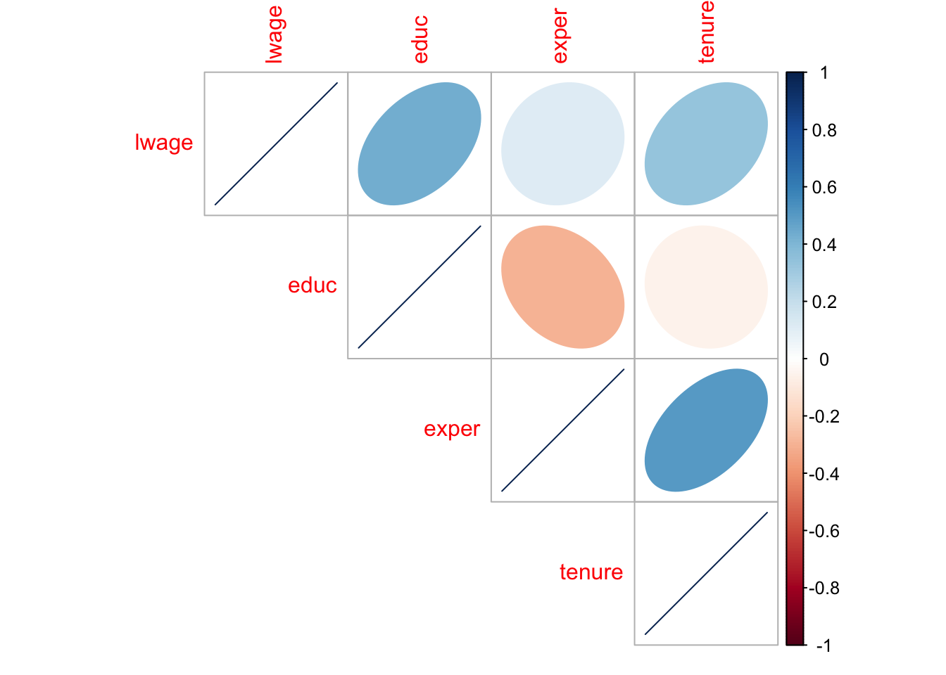
Figure 4.3: correlation plot
The way to read the so-called correlation plot in figure 4.3 is straightforward: each row illustrates the correlation of a certain variable with the other variables. In this example both the shape of the ellipse in each cell as well as their color coding tell us how strongly two variables correlate. Let us put this into a regression model now:
educ_only <- lm(lwage ~ educ                 , data = wage1)
educ_exper <- lm(lwage ~ educ + exper        , data = wage1)
log_wages <- lm(lwage ~ educ + exper + tenure, data = wage1)
stargazer::stargazer(educ_only, educ_exper, log_wages,type = if (knitr:::is_latex_output()) "latex" else "html")| Dependent variable: | |||
| lwage | |||
| (1) | (2) | (3) | |
| educ | 0.083*** | 0.098*** | 0.092*** |
| (0.008) | (0.008) | (0.007) | |
| exper | 0.010*** | 0.004** | |
| (0.002) | (0.002) | ||
| tenure | 0.022*** | ||
| (0.003) | |||
| Constant | 0.584*** | 0.217** | 0.284*** |
| (0.097) | (0.109) | (0.104) | |
| Observations | 526 | 526 | 526 |
| R2 | 0.186 | 0.249 | 0.316 |
| Adjusted R2 | 0.184 | 0.246 | 0.312 |
| Residual Std. Error | 0.480 (df = 524) | 0.461 (df = 523) | 0.441 (df = 522) |
| F Statistic | 119.582*** (df = 1; 524) | 86.862*** (df = 2; 523) | 80.391*** (df = 3; 522) |
| Note: | p<0.1; p<0.05; p<0.01 | ||
Column (1) refers to model (3.16) from the previous chapter, where we only had educ as a regressor: we obtain an \(R^2\) of 0.186. Column (2) is the model that generated the plane in figure 4.2 above. (3) is the model with three regressors. You can see that by adding more regressors, the quality of our fit increases, as more of the variation in \(y\) is now accounted for by our model. You can also see that the values of our estimated coefficients keeps changing as we move from left to right across the columns. Given the correlation structure shown in figure 4.3, it is only natural that this is happening: We see that educ and exper are negatively correlated, for example. So, if we omit exper from the model in column (1), educ will reflect part of this correlation with exper by a lower estimated value. By directly controlling for exper in column (2) we get an estimate of the effect of educ net of whatever effect exper has in isolation on the outcome variable. We will come back to this point later on.
4.4 How To Make Predictions
So suppose we have a model like
\[\text{lwage} = b_0 + b_{1}(\text{educ}) + b_{2}(\text{exper}) + b_{3}(\text{tenure}) + \epsilon\]
How could we use this to make a prediction of log wages, given some new data? Remember that the OLS procedure gives us estimates for the values \(b_0,b_1, b_2,b_3\). With those in hand, it is straightforward to make a prediction about the conditional mean of the outcome - just plug in the desired numbers for educ,exper and tenure. Suppose you want to know what the mean of lwage is conditional on educ = 10,exper=4 and tenure = 2. You’d do
\[\begin{align} E[\text{lwage}|\text{educ}=10,\text{exper}=4,\text{tenure}=2] &= b_0 + b_1 10 + b_2 4 + b_3 2\\ &= 1.27. \end{align}\]
I computed the last line directly with
but R has a more complete prediction interface, using the function predict. For starters, you can predict the model on all data points which were contained in the dataset we used for estimation, i.e. wage1 in our case:
##        1        2        3        4        5        6
## 1.304921 1.523506 1.304921 1.819802 1.461690 1.970451
Often you want to add that prediction to the original dataset:
wage_prediction = cbind(wage1, prediction = predict(log_wages))
head(wage_prediction[, c("lwage","educ","exper","tenure","prediction")])
## lwage educ exper tenure prediction
## 1 1.131402 11 2 0 1.304921
## 2 1.175573 12 22 2 1.523506
## 3 1.098612 11 2 0 1.304921
## 4 1.791759 8 44 28 1.819802
## 5 1.667707 12 7 2 1.461690
## 6 2.169054 16 9 8 1.970451You’ll remember that we called the distance in prediction and observed outcome our residual \(e\). Well here this is just lwage - prediction. Indeed, \(e\) is such an important quantity that R has a convenient method to compute \(y - \hat{y}\) from an lm object directly - the method resid. Let’s add another column to wage_prediction:
wage_prediction = cbind(wage_prediction, residual = resid(log_wages))
head(wage_prediction[, c("lwage","educ","exper","tenure","prediction","residual")])
## lwage educ exper tenure prediction residual
## 1 1.131402 11 2 0 1.304921 -0.17351850
## 2 1.175573 12 22 2 1.523506 -0.34793289
## 3 1.098612 11 2 0 1.304921 -0.20630832
## 4 1.791759 8 44 28 1.819802 -0.02804286
## 5 1.667707 12 7 2 1.461690 0.20601725
## 6 2.169054 16 9 8 1.970451 0.19860271Using the data in wage_prediction, you should now check for yourself what we already know about \(\hat{y}\) and \(e\) from section 3.3:
- What is the average of the vector
residual? - What is the average of
prediction? - How does this compare to the average of the outcome
lwage? - What is the correlation between
predictionandresidual?