Chapter 11 IV Applications

An important term in economics are the returns to schooling, by which we mean the causal effect of education on later earnings. If you think about it, it’s a crucial question for every single student (like yourself), if not even more so for a policy maker who needs to decide where to allocate budget spending on (education or other things?).

One very famous and early study to estimate those returns to schooling was proposed by Jacob Mincer, and an equation of this kind was henceforth known as the Mincer Equation (we have encountered this equation before as a running example in chapter 3). He measured \(\log Y_i\), annual earnings for man \(i\), \(S_i\) his schooling (years spent studying), and \(X_i\) his (potential) work experience (age minus years of schooling minus 6). The model can be drawn like this:

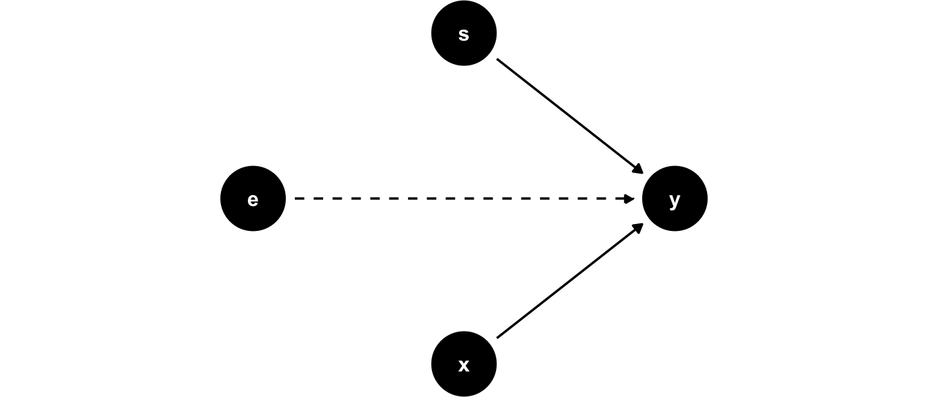
Figure 11.1: Jacob Mincer’s model

Hourly earnings are assumed to be affected by experience and schooling only. In terms of an equation,

\[\begin{equation} \log Y_i = \alpha + \rho S_i + \beta_1 X_i + \beta_2 X_i^2 + e_i \tag{11.1} \end{equation}\]

His results implied an estimate for \(\rho\) of about 0.11, or an 11% earnings advantage for each additional year of education, given a certain level of experience. Notice that in the DAG in figure 11.1, we explicitly drew other unobserved factors \(e\) with only have an arrow directly into \(y\). But is that a good model? Well, why would it not be?

11.1 Ability Bias

The model in (11.1) compares earnings of men with certain schooling and work experience. The question to ask, if given those two controls, all else is equal? For a given value of \(X\), are there more diligent and able workers out there? Do family connections vary across people with the same \(X\)? It seems quite likely that we’d answer yes. Well, then, all else is not equal, and we are in trouble. Because, again, our crucial identifying assumption for the linear model is violated, as

\[E[e_i | S_i, X_i] \neq 0.\]

Our concern can be formalized by explicitly introducing ability \(A\) as an (unobserved) factor into our model. That means we have now two unobservables - of course we can’t tell them apart, so let’s write them as a new unobservable factor \(u_i = e_i + A_i\). Then we could visualize this new model as follows:

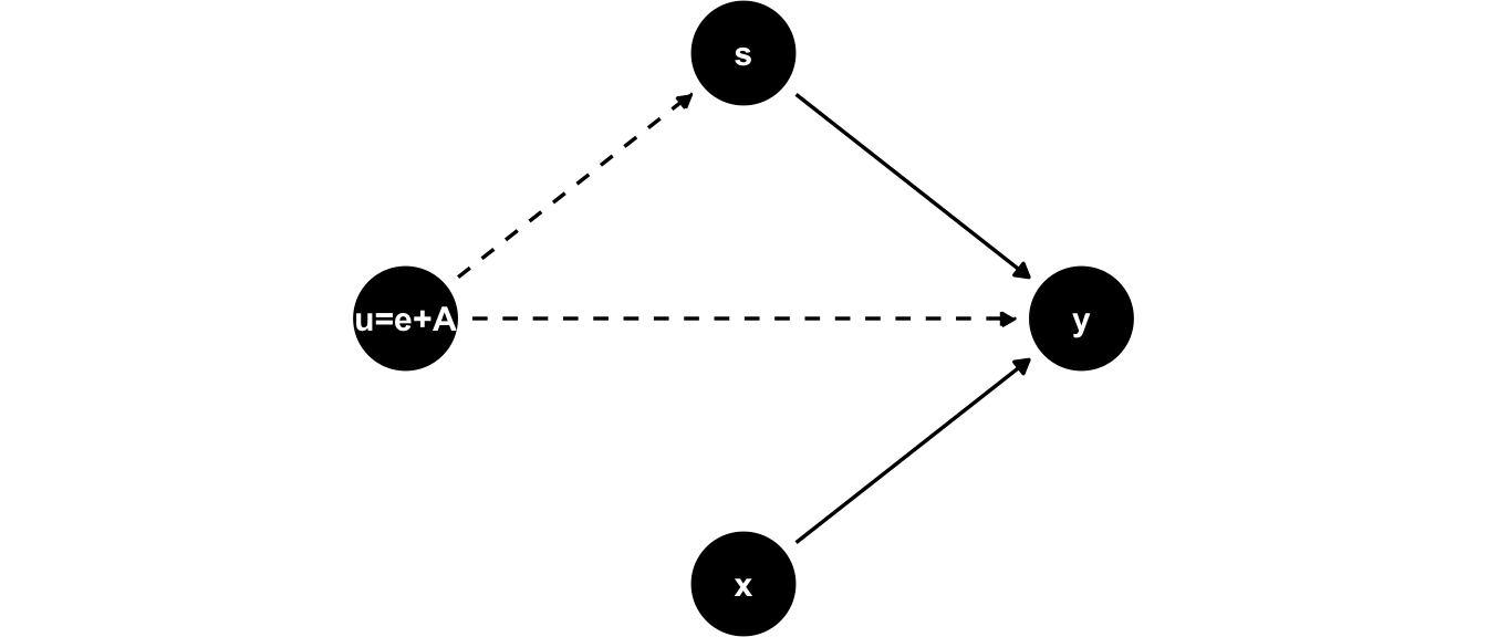
Figure 11.2: Jacob Mincer’s model with unobserved ability \(A\). Given it’s unobserved it is lumped together with all other unobservable factors in \(e\), and we’ve called it \(u = e + A\).

In figure 11.2, the unobserved factor \(A\) influences both years of schooling and earnings on the labor market. For example, if we think for \(A\) as something like intelligence, it might be that more intelligent students find it less painful to attend school (it’s less costly for them in terms of effort), so they get more education, and also they earn higher wages because their intelligence is rewarded in the labor market. The same works if \(A\) is related to family type and network. Suppose a family with high socio-economic status is also well connected. Then high \(A\) could mean that the parents of \(i\) know that education is a good signalling device (so they force \(i\) to go to university, say), while at the same time their good network means that high \(A\) will mean a good job and hence earnings. We would write in terms of an equation

\[\begin{equation} \log Y_i = \alpha + \rho S_i + \beta_1 X_i + \beta_2 X_i^2 + \underbrace{u_i}_{A_i + e_i} \tag{11.2} \end{equation}\]

Sometimes these considerations do not matter greatly, and the (biased) OLS estimate is close the causal IV estimate. But in other cases, we might be very far from the truth with OLS, even inferring the wrong sign of an effect. Let’s look at an example!

11.2 Birthdate is as good as Random

In an influential study, Angrist and Krueger (1991) address the above issues related to the ability bias in Mincer’s equation by constructing an IV which encodes the birth date of a given student. The idea is that given certain features of the school system, children born shortly after a certain cutoff date will start school a year later than their peers who are a bit older than they are.

For example, suppose it is mandated that all children who reach the age of 6 by 31st of december 2021 are required to enroll in the first grade of school in september 2021. Then someone born in September 2015 (i.e. 6 years prior) will be 5 years and 3/4 by the time they start school, while someone born on the 1st of January 2016 will be 6 and 3/4 years when they enter school in september 2022. Furthermore, the legal dropout age in the US is 16, so by the time those pupils may decide to stop school, they have been exposed to different amounts of schooling. All of this means that an IV defined by quarter of birth of person \(i\) will affect the outcome earnings through it’s effect on more schooling - keeping other factors (in particular \(A\)!) constant across values of the IV. What’s the implication for our model?

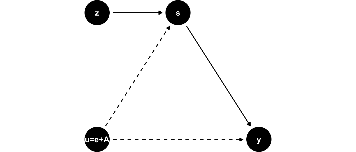
Figure 11.3: Angrist and Krueger’s IV in to tackle ability bias.

In the DAG for Angrist and Krueger (1991)’s model in 11.3 we see that the IV directly impacts the endogenous explanatory variable \(s\), but is itself independent of \(u\) - we argued that \(A\) is equally distributed across different birth quarters \(z\) (birth date is almost random). Let us now formulate the following two-stage procedure:

1. We estimate a first stage model which uses only exogenous variables (like \(z\)) to explain our endgenous regressor \(s\).
2. We then use the first stage model to predict values of \(s\) in what is called the second stage or the reduced form model.¹³ Performing this procedure is supposed to take out any impact of \(A\) in the correlation we observe in our data between \(s\) and \(y\).

This estimation technique is called the Two stage least squares estimator, or 2SLS for short. The great virtue is that in the first stage we could have any number of exogenous variables helping to predict our exogenous \(s\) (here we have just one - quarter of birth.) In terms of equations, we could write the following:

\[\begin{align} \text{1. Stage: }s_i &= \alpha_0 + \alpha_1 z_i + \eta_i \tag{11.3}\\ \text{2. Stage: }y_i &= \beta_0 + \beta_1 \hat{s}_i + u_i \tag{11.4} \end{align}\]

where the \(\hat{s}_i\) means to insert the predicted value from the first stage for \(i\)’s observed \(s_i\) in the second stage regression. We can write down the conditions for a valid IV \(z\) in this context:

Conditions for a valid Instrument in this simple 2SLS setup:

1. Relevance of the IV: \(\alpha_1 \neq 0\)
2. Independence (IV assignment as good as random): \(E[\eta | z] = 0\)
3. Exogeneity (our exclusion restriction): \(E[u | z] = 0\)

11.2.1 Data on birth quarter and wages

Let’s load the data and look at a quick summary¹⁴:

data("ak91", package = "masteringmetrics")
# library(modelsummary) # loaded already for me
datasummary_skim(data.frame(ak91),histogram = TRUE)

	Unique (#)	Missing (%)	Mean	SD	Min	Median	Max
lnw	26732	0	5.9	0.7	-2.3	6.0	10.5
s	21	0	12.8	3.3	0.0	12.0	20.0
yob	10	0	1934.6	2.9	1930.0	1935.0	1939.0
qob	4	0	2.5	1.1	1.0	3.0	4.0
sob	51	0	30.7	14.2	1.0	34.0	56.0
age	40	0	45.0	2.9	40.2	45.0	50.0

We convert quarter of birth to a factor:

ak91 <- mutate(ak91,
               qob_fct = factor(qob),
               q4 = as.integer(qob == "4"),
               yob_fct = factor(yob))
# get mean wage by year/quarter
ak91_age <- ak91 %>%
  group_by(qob, yob) %>%
  summarise(lnw = mean(lnw), s = mean(s)) %>%
  mutate(q4 = (qob == 4))

## `summarise()` regrouping output by 'qob' (override with `.groups` argument)

Let’s reproduce their first figure now on education as a function of quarter of birth!

ggplot(ak91_age, aes(x = yob + (qob - 1) / 4, y = s )) +
  geom_line() + 
  geom_label(mapping = aes(label = qob, color = q4)) +
  guides(label = FALSE, color = FALSE) +
  scale_x_continuous("Year of birth", breaks = 1930:1940) +
  scale_y_continuous("Years of Education", breaks = seq(12.2, 13.2, by = 0.2),
                     limits = c(12.2, 13.2)) +
  theme_bw()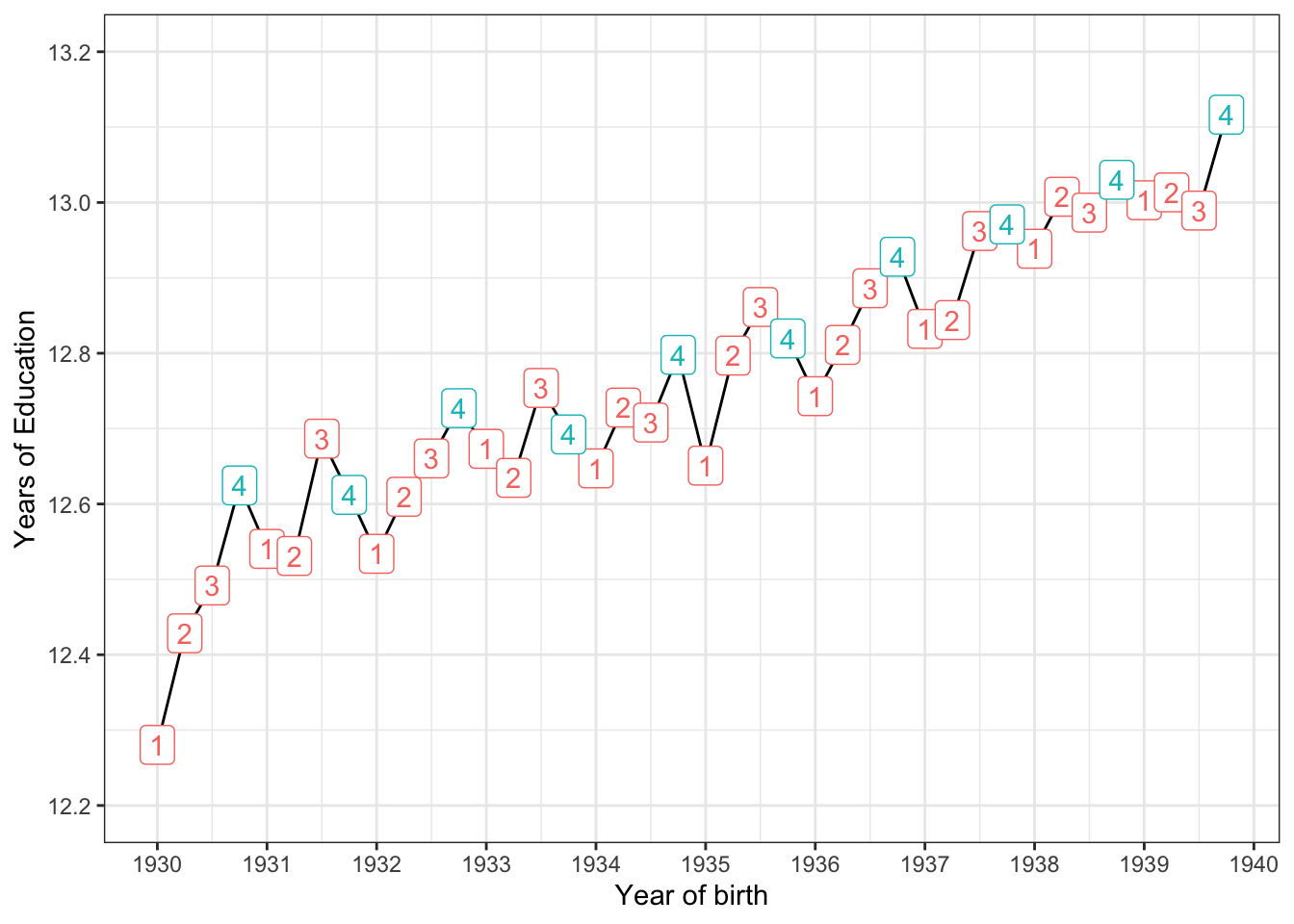

Figure 11.4: Reproducing figure 1 from Angrist and Krueger (2001)

In figure 11.4 we see first that there was a trend in getting more and more education as time passed. Secondly, and more importantly here, is that for almost all birth years in the sample, the group born in quarter 4 has the highest value for years of education! So what we said above about the instutional rules of school attendance in the US seems to be born out in this dataset. What about earnings for those groups?

ggplot(ak91_age, aes(x = yob + (qob - 1) / 4, y = lnw)) +
  geom_line() +
  geom_label(mapping = aes(label = qob, color = q4)) +
  scale_x_continuous("Year of birth", breaks = 1930:1940) +
  scale_y_continuous("Log weekly wages") +
  guides(label = FALSE, color = FALSE) +  
  theme_bw()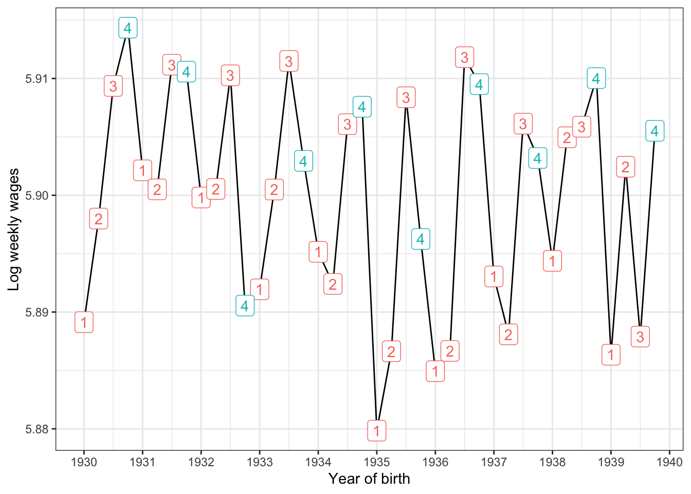

Figure 11.5: Reproducing figure 2 from Angrist and Krueger (2001)

Figure 11.5 does not show a long running trend in earnings, so on average we’d say an hourly wage of 5 Dollars 90 per week. But, again, the group born in the fourth quarter seems special: In many cases they earn the highest or close to highest wage if compared to the other 3 groups in their birthyear. So, there really seems to be a relationship between quarter of birth and later in life earnings! Let us now construct an IV estimator, which will allow us to relate the sawtooth pattern in figure 11.4 to the one in 11.5. We will start out with using just born in fourth quarter as our IV.

11.2.2 Running IV estimation in R

There are several possibilities to run IV estimation in R. We will use the iv_robust function from the estimatr package.¹⁵ Let’s estimate a simple OLS version (subject to ability bias), the first stage and second stages, and the final 2SLS estimate:

mod                  <- list()
mod$ols              <- lm(lnw ~ s, data = ak91)
mod[["first stage"]] <- lm(s ~ q4, data = ak91)  # IV: born in q4 is TRUE?
ak91$shat            <- predict(mod[["first stage"]])  
mod[["second stage"]] <- lm(lnw ~ shat, data = ak91)
mod$`2SLS`            <- estimatr::iv_robust(lnw ~ s | q4, data = ak91 ) # IV: born in q4 is TRUE?

Let’s look at those models next to each other in table 11.1:

Table 11.1: OLS, first and sceond stages as well as 2SLS estimates for Angrist and Krueger (1991)

	ols	first stage	second stage	2SLS
(Intercept)	4.995***	12.747***	4.955***	4.955***
	(0.004)	(0.007)	(0.381)	(0.358)
s	0.071***			0.074***
	(0.000)			(0.028)
q4		0.092***
		(0.013)
shat			0.074**
			(0.030)
F	43782.556	48.095	6.146
* p < 0.1, ** p < 0.05, *** p < 0.01

Table 11.1 contains a lot of information, so let’s go column-wise:

1. The column labelled ols is the basic earnings equation similar to Mincer’s model (without experience). We are worried about bias from the omitted variable ability, but we note that here we estimate a 7% higher wage for each additional year of schooling.
2. The next column is the first stage, i.e. the estimates for \(\alpha\) in equation (11.3). Remember we require that \(\alpha_1 \neq 0\). That seems to be the case here (p-value very small).
3. Then we run the second stage model with the predicted values \(\hat{s}\) from the first stage, i.e. we estimate the \(\beta\)s in (11.4). You should compare s and shat in the first and third column.
4. Finally, we perform first and second stag e estimation in one go (you would usually go down this route directly) with 2SLS. You should compare shat from the second stage with the s estimate from the 2SLS model! The reason you should always go directly to something like iv_robust is that this procedure handles computation of standard errors correctly. In other words, the displayed standard error in the second stage for shat (0.03) is not taking into account that we estimated shat itself in a previous step - iv_robust does (note the small difference to 0.028).

11.2.3 Additional Control Variables

We saw in figure 11.4 that there is a clear time trend in years of schooling. There are also business-cycle fluctuations in earnings, even if we were not able to see them from the graph above. It is probably a good idea to control for calendar year in order to guard against any time effects in our results. Also, we can use more than one IV! Here is how:

mod$ols_yr  <- update(mod$ols, . ~ . + yob_fct)  # just update previous model
mod[["2SLS_yr"]] <- estimatr::iv_robust(lnw ~ s  + yob_fct | q4 + yob_fct, data = ak91 )  # add exogenous vars on both sides of | !
mod[["2SLS_all"]] <- estimatr::iv_robust(lnw ~ s  + yob_fct | qob_fct + yob_fct, data = ak91 )  # use all quarters as IVs

# here is how to make the table:
rows <- data.frame(term = c("Instruments","Year of birth"),
                   ols  = c("none","no"),
                   SLS  = c("Q4","no"),
                   ols_yr  = c("none","yes"),
                   SLS_yr  = c("Q4","yes"),
                   SLS_all  = c("All Quarters","yes")
                   )
names(rows)[c(3,5,6)] <- c("2SLS","2SLS_yr","2SLS_all")
modelsummary::msummary(models = mod[c("ols","2SLS","ols_yr","2SLS_yr","2SLS_all")], 
                       statistic = 'std.error',
                       gof_omit = 'DF|Deviance|AIC|BIC|R2|p.value|se_type|statistic|Log.Lik.|Num.Obs.|N',
                       title = "Adding Year as control, and more IVs",
                       add_rows = rows,
                       coef_omit = 'yob_fct')

Table 11.2: Adding Year as control, and more IVs

	ols	2SLS	ols_yr	2SLS_yr	2SLS_all
(Intercept)	4.995	4.955	5.017	4.966	4.592
	(0.004)	(0.358)	(0.005)	(0.354)	(0.251)
s	0.071	0.074	0.071	0.075	0.105
	(0.000)	(0.028)	(0.000)	(0.028)	(0.020)
F	43782.556		4397.455
Instruments	none	Q4	none	Q4	All Quarters
Year of birth	no	no	yes	yes	yes

11.3 IV Mechanics

Let’s now look a little closer under the hood of our simple IV estimator. We want to understand how inference of IV relates to OLS inference, and what we can say about weak instruments, i.e. IVs with small predictive power in the first stage.

Let’s go back to our simple linear model

\[ y = \beta_0 + \beta_1 x + u \tag{11.5} \]

where we think that \(Cov(x,u) \neq 0\), hence, that \(x\) is endogenous in this equation. By the way, IV estimation will work whether or not \(Cov(x,u) \neq 0\), but we should prefer OLS if \(x\) is exogenous, as should become clear soon.

We now know that the conditions under which IV \(z\) will deliver consistent estimates are the following:

1. first stage or relevance: \(Cov(z,x) \neq 0\)
2. IV exogeneity: \(Cov(z,u) = 0\): the IV is exogenous in the outcome equation.

To reiterate, condition 2 here calls for \(z\) to have no partial effect on \(y\), after \(x\) and other omitted variables have been considered (they are in \(u\)), hence, that \(z\) is uncorrelated with \(u\). Figure 11.6 shows a valid IV in panel A and an IV which violates condition 2 in panel B.

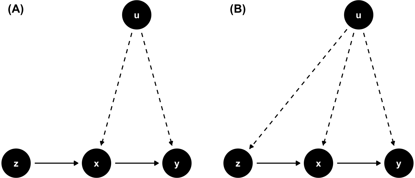
Figure 11.6: A valid IV (A) and one where the exogeneity assumption is violated (B).

Let us now discuss how conditions 1. and 2. are helpful in identifying parameter \(\beta_1\) above. By this we mean our ability to express \(\beta_1\) in terms of population moments, which we can estimate from a sample of data. We start by computing the covariance of the instrument \(z\) with outcome \(y\).

\[\begin{align} Cov(z,y) &= Cov(z, \beta_0 + \beta_1 x + u) \\ &= \beta_1 Cov(z,x) + Cov(z,u) \end{align}\]

Under condition 2. above (IV exogeneity), we have \(Cov(z,u)=0\), hence

\[ Cov(z,y) = \beta_1 Cov(z,x) \] and under condition 1. (relevance), we have \(Cov(z,x)\neq0\), so that we can divide the equation through to obtain

\[ \beta_1 = \frac{Cov(z,y)}{Cov(z,x)}. \] This shows that the parameter \(\beta_1\) is identified via population moments \(Cov(z,y)\) and \(Cov(z,x)\). What is more, we can estimate those moments via their sample analogs, hence we have as an IV estimator this expression, where we just plug in the sample estimators for the population moments:

\[ \hat{\beta}_1 = \frac{\sum_{i=1}^n (z_i - \bar{z})(y_i - \bar{y})}{\sum_{i=1}^n (z_i - \bar{z})(x_i - \bar{x})} \tag{11.6} \] The corresponding intercept estimate \(\hat{\beta}_0 = \bar{y} - \hat{\beta}_1 \bar{x}\) is identical to before (modulo using (11.6)).

Given both assumptions 1. and 2. are satisfied, we say that the IV estimator is consistent for \(\beta_1\). This can also be written as

\[ \text{plim}(\hat{\beta}_1) = \beta_1 \]

meaning that, as the sample size \(n\) increases, the probability limit (plim) of the estimator \(\hat{\beta}_1\) is the true value \(\beta_1\).¹⁶

11.3.1 IV Inference

Let us extend the homoskedasticity assumption to \(z\), such that \(E(u^2|z) = \sigma^2\), implying that the asymptotic (i.e. as the sample size gets very large) variance of the IV slope estimator is given by

\[ Var(\hat{\beta}_{1,IV}) = \frac{\sigma^2}{n \sigma_x^2 \rho_{x,z}^2} \tag{11.7} \] where \(\sigma_x^2\) is the population variance of \(x\), \(\sigma^2\) the one of \(u\), and \(\rho_{x,z}\) is the population correlation between \(x\) and \(z\) - a measure of how strongly our IV and endogenous variable \(x\) are correlated in the population.

You can see 2 important things in equation (11.7):

1. Without the term \(\rho_{x,z}^2\) in the denominator, this is identical to the variance of the OLS slope estimator.
2. As with the variance of the OLS slope estimator, as sample size \(n\) increases, the variance decreases.

It is convenient to replace \(\rho_{x,z}^2\) with \(R_{x,z}^2\), i.e. the R-squared of a regression of \(x\) on \(z\) - in a single regressor model we have this exact correspondence. It is convenient because we rewrite the variance of the IV slope now as

\[ Var(\hat{\beta}_{1,IV}) = \frac{\sigma^2}{n \sigma_x^2 R_{x,z}^2} \]

1. Given \(R_{x,z}^2 < 1\) in most real life situations, we have that \(Var(\hat{\beta}_{1,IV}) > Var(\hat{\beta}_{1,OLS})\) almost certainly.
2. The higher the correlation between \(z\) and \(x\), the closer their \(R_{x,z}^2\) is to 1. With \(R_{x,z}^2 = 1\) we get back to the OLS variance. This is no surprise, because that implies that in fact \(z = x\).

So, if you have a valid, exogenous regressor \(x\), you should not perform IV estimation using \(z\) to obtain \(\hat{\beta}\), since your variance will be unnecessarily large.

11.3.1.1 Returns to Education for Married Women

Consider the following model for married women’s wages:

\[ \log wage = \beta_0 + \beta_1 educ + u \] Let’s run an OLS on this, and then compare it to an IV estimate using father’s education. Keep in mind that this is a valid IV \(z\) if

1. fatheduc and educ are correlated
2. fatheduc and \(u\) are not correlated.

data(mroz,package = "wooldridge")
mods = list()
mods$OLS <- lm(lwage ~ educ, data = mroz)
mods[['First Stage']] <- lm(educ ~ fatheduc, data = subset(mroz, inlf == 1))
mods$IV  <- estimatr::iv_robust(lwage ~ educ | fatheduc, data = mroz)
modelsummary::modelsummary(mods, gof_map = gm, 
                           gof_omit = gom, 
                           title = "Mroz female labor supply and wage data.")

Table 11.3: Mroz female labor supply and wage data.

	OLS	First Stage	IV
(Intercept)	-0.185	10.237	0.441
	(0.185)	(0.276)	(0.467)
educ	0.109		0.059
	(0.014)		(0.037)
fatheduc		0.269
		(0.029)
Num.Obs.	428	428	428
R2	0.118	0.173	0.093

The results in table 11.3 show in the first column that an additional year of education implies an 11% increase in annual wages for women. This is a standard OLS estimator which be biased because of ability bias.

In the second column we show the first stage of the IV procedure. We see that fatheduc is indeed a statistically significant predictor of \(educ\): Each additional year of father’s education increases women’s education by more than a quarter of a year (0.269). Also important, we observe that the \(R^2\) here is about 17%.

Turning to the final IV estimate in the third column, we can see that using fatheduc as an IV reduces the return to education by about half to 5.9%! This result suggests that OLS is biased upwards (for example by ability bias). But let’s compare the standard errors of OLS and IV estimates, which are 0.014 for OLS vs 0.037 for IV. This can be seen in figure 11.7. You can clearly see that the standard errors of both estimators overlap, hence from this alone we cannot conclude they are different (we need a special statistical test to decide this).

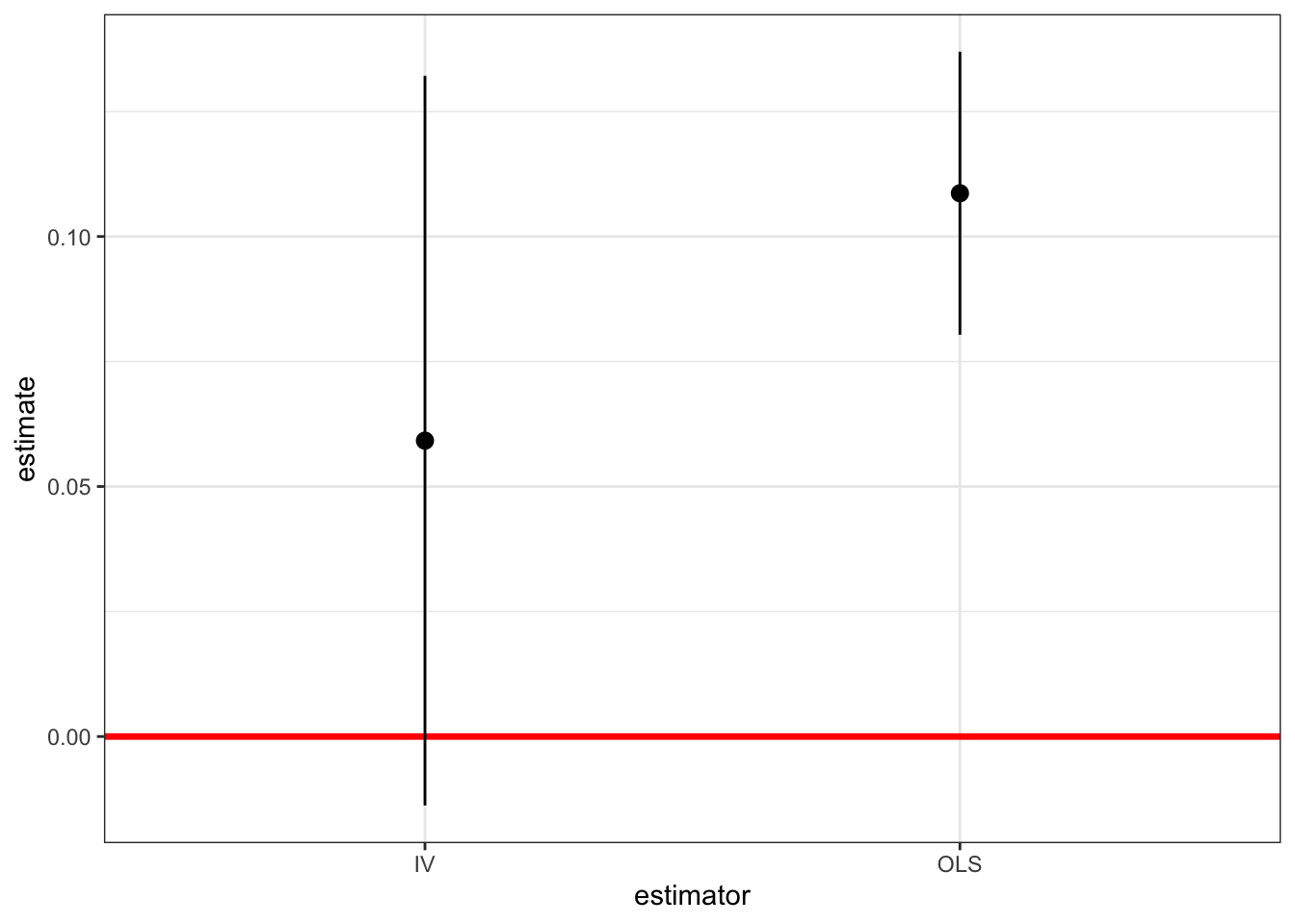
Figure 11.7: OLS vs IV Standard Errors: The dots represent the point estimates, and the solid vertical lines the standard error for both estimators.

11.3.2 IV with a Weak Instrument

We have seen that IV will produce consistent estimates under our stated assumptions. However, even under valid assumption, we get large IV standard errors if the the correlation between IV and endogenous \(x\) is small.
What is even worse is that even if we have only very small correlation between \(z\) and \(u\), so that we might almost be happy to assume exogeneity, a small corrleation between \(x\) and \(z\) can produce inconsistent estimates. To see this, consider the probability limit of the IV estimator again

\[ \text{plim}(\hat{\beta}_{1,IV}) = \beta_1 + \frac{Cor(z,u)}{Cor(z,x)} \cdot \frac{\sigma_u}{\sigma_x} \]

The interesting part here involves the correlation terms. Even if \(Cor(z,u)\) is very small, a weak instrument, i.e. one with only a small absolute value for \(Cor(z,x)\) will blow up this second term in the probability limit. This would mean that even with a very big sample size \(n\), our estimator would not converge to the true population parameter \(\beta_1\), because we are using a weak instrument.

To illustrate this point, let’s assume we want to look at the impact of number of packs of cigarettes smoked per day by pregnant women (packs) on the birthweight of their child (bwght):

\[ \log(bwght) = \beta_0 + \beta_1 packs + u \]

We are worried that smoking behavior is correlated with a range of other health-related variables which are in \(u\) and which could impact the birthweight of the child - think of diet, physical exercise, and other lifestyle choices. So we look for an IV. Suppose we use the price of cigarettes (cigprice), assuming that the price of cigarettes is uncorrelated with factors in \(u\) - the price of cigarettes would not impact birthweight (apart from through its effect on smoking behaviour, of course). Let’s run the first stage of cigprice on packs and then let’s show the 2SLS estimates:

data(bwght, package = "wooldridge")
mods <- list()
mods[["First Stage"]] <- lm(packs ~ cigprice, data = bwght)
mods[["IV"]] <- estimatr::iv_robust(log(bwght) ~  packs | cigprice, data = bwght)
modelsummary(mods, gof_map = gm, 
             gof_omit = gom, 
             title = "IV regression with weak instrument *cigprice*")

Table 11.4: IV regression with weak instrument cigprice

	First Stage	IV
(Intercept)	0.067	4.448
	(0.103)	(0.940)
cigprice	0.000
	(0.001)
packs		2.989
		(8.996)
Num.Obs.	1388	1388
R2	0.000	-23.230

The first column of table 11.4 shows that the first stage is very weak. The partial effect of cigprice on packs smoked is zero! People don’t seem to care a great deal about the price of cigarettes (at least in the range of price variation observed in this dataset). The \(R^2\) of that first stage is thus zero. What do we get if we use that IV nonetheless in a 2SLS estimation as in column 2? We get a huge coefficient of unexpected sign on packs (smoking more increases birthweight? 🤔), with very large standard error, so statistically speaking, we cannot distinguish this from zero. What is more important, however, is that even if they were significant, the estimates of column 2 are invalid. The relevance of the IV condition is clearly not satisfied, hence, invalid approach. ⛔

References

Angrist, Joshua D, and Alan B Krueger. 2001. “Instrumental Variables and the Search for Identification: From Supply and Demand to Natural Experiments.” Journal of Economic Perspectives 15 (4): 69–85.

Angrist, Joshua D., and Alan B. Krueger. 1991. “Does Compulsory School Attendance Affect Schooling and Earnings?” The Quarterly Journal of Economics 106 (4): 979–1014. https://doi.org/10.2307/2937954.

---

13. It’s called reduced form because this second equation is supposed to be derived from a true underlying structural model.↩︎

14. Code in this section comes from the great mastering metrics with R by J Arnold 👏 🙏↩︎

15. the robust here refers to the fact that the estimatr package by default chooses formulae to compute standard errors which are correcting for heteroskedasticity - we have encountered this term before in 6.6.2. See details here↩︎

16. More precisely, we say that a sequence of random variables indexed by sample size \(n\), \({X_n}\) say, converges in probability to the random variable \(X\), if for all \(\varepsilon > 0\), \[ \lim_{n \to \infty} \Pr \left(|X_n - X | > \varepsilon \right) = 0 \]↩︎